|
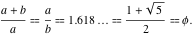
The division of a line segment whose total length is a + b into two parts a and b where the ratio of a + b to a is equal to the ratio a to b is known as the golden ratio. The two ratios are both approximately equal to 1.618..., which is called the golden ratio constant and usually notated by  : :

|
The concept of golden ratio division appeared more than 2400 years ago as evidenced in art and architecture. It is possible that the magical golden ratio divisions of parts are rather closely associated with the notion of beauty in pleasing, harmonious proportions expressed in different areas of knowledge by biologists, artists, musicians, historians, architects, psychologists, scientists, and even mystics. For example, the Greek sculptor Phidias (490–430 BC) made the Parthenon statues in a way that seems to embody the golden ratio; Plato (427–347 BC), in his Timaeus, describes the five possible regular solids, known as the Platonic solids (the tetrahedron, cube, octahedron, dodecahedron, and icosahedron), some of which are related to the golden ratio.
The properties of the golden ratio were mentioned in the works of the ancient Greeks Pythagoras (c. 580–c. 500 BC) and Euclid (c. 325–c. 265 BC), the Italian mathematician Leonardo of Pisa (1170s or 1180s–1250), and the Renaissance astronomer J. Kepler (1571–1630). Specifically, in book VI of the Elements, Euclid gave the following definition of the golden ratio: "A straight line is said to have been cut in extreme and mean ratio when, as the whole line is to the greater segment, so is the greater to the less". Therein Euclid showed that the "mean and extreme ratio", the name used for the golden ratio until about the 18th century, is an irrational number.
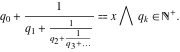
In 1509 L. Pacioli published the book De Divina Proportione, which gave new impetus to the theory of the golden ratio; in particular, he illustrated the golden ratio as applied to human faces by artists, architects, scientists, and mystics. G. Cardano (1545) mentioned the golden ratio in his famous book Ars Magna, where he solved quadratic and cubic equations and was the first to explicitly make calculations with complex numbers. Later M. Mästlin (1597) evaluated  approximately as approximately as  . J. Kepler (1608) showed that the ratios of Fibonacci numbers approximate the value of the golden ratio and described the golden ratio as a "precious jewel". R. Simson (1753) gave a simple limit representation of the golden ratio based on its very simple continued fraction . J. Kepler (1608) showed that the ratios of Fibonacci numbers approximate the value of the golden ratio and described the golden ratio as a "precious jewel". R. Simson (1753) gave a simple limit representation of the golden ratio based on its very simple continued fraction  . M. Ohm (1835) gave the first known use of the term "golden section", believed to have originated earlier in the century from an unknown source. J. Sulley (1875) first used the term "golden ratio" in English and G. Chrystal (1898) first used this term in a mathematical context. . M. Ohm (1835) gave the first known use of the term "golden section", believed to have originated earlier in the century from an unknown source. J. Sulley (1875) first used the term "golden ratio" in English and G. Chrystal (1898) first used this term in a mathematical context.
The symbol  (phi) for the notation of the golden ratio was suggested by American mathematician M. Barrwas in 1909. Phi is the first Greek letter in the name of the Greek sculptor Phidias. (phi) for the notation of the golden ratio was suggested by American mathematician M. Barrwas in 1909. Phi is the first Greek letter in the name of the Greek sculptor Phidias.
Throughout history many people have tried to attribute some kind of magic or cult meaning as a valid description of nature and attempted to prove that the golden ratio was incorporated into different architecture and art objects (like the Great Pyramid, the Parthenon, old buildings, sculptures and pictures). But modern investigations (for example, G. Markowsky (1992), C. Falbo (2005), and A. Olariu (2007)) showed that these are mostly misconceptions: the differences between the golden ratio and real ratios of these objects in many cases reach 20–30% or more.
The golden ratio has many remarkable properties related to its quasi symmetry. It satisfies the quadratic equation  , which has solutions , which has solutions  and and  . The absolute value of the second solution is called the golden ratio conjugate, . The absolute value of the second solution is called the golden ratio conjugate,  . These ratios satisfy the following relations: . These ratios satisfy the following relations:
Applications of the golden ratio also include algebraic coding theory, linear sequential circuits, quasicrystals, phyllotaxis, biomathematics, and computer science.
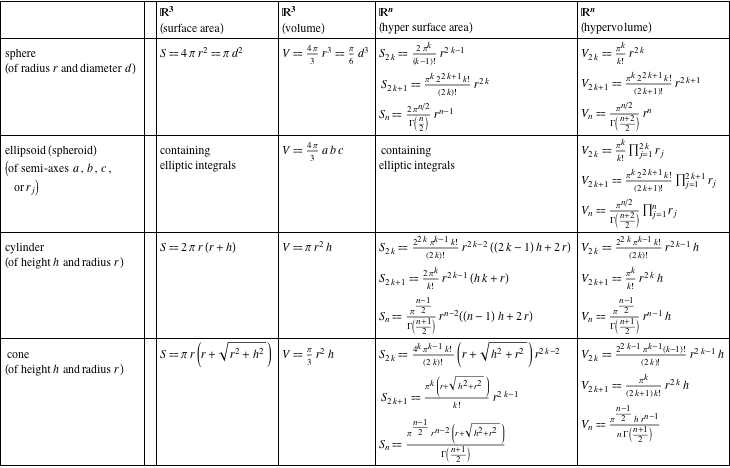
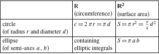
The constant  is the most frequently encountered classical constant in mathematics and the natural sciences. Initially it was defined as the ratio of the length of a circle's circumference to its diameter. Many further interpretations and applications in practically all fields of qualitative science followed. For instance, the following table illustrates how the constant is the most frequently encountered classical constant in mathematics and the natural sciences. Initially it was defined as the ratio of the length of a circle's circumference to its diameter. Many further interpretations and applications in practically all fields of qualitative science followed. For instance, the following table illustrates how the constant  is applied to evaluate surface areas and volumes of some simple geometrical objects: is applied to evaluate surface areas and volumes of some simple geometrical objects:
|
|
Different approximations of π have been known since antiquity or before when people discovered some basic properties of circles. The design of Egyptian pyramids (c. 3000 BC) incorporated  as as  in numerous places. The Egyptian scribe Ahmes (Middle Kingdom papyrus, c. 2000 BC) wrote the oldest known text to give an approximate value for in numerous places. The Egyptian scribe Ahmes (Middle Kingdom papyrus, c. 2000 BC) wrote the oldest known text to give an approximate value for  as as 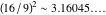 Babylonian mathematicians (19th century BC) were using an estimation of π as Babylonian mathematicians (19th century BC) were using an estimation of π as  , which is within 0.53% of the exact value. (China, c. 1200 BC) and the Biblical verse I Kings 7:23 (c. 971–852 BC) gave the estimation of π as 3. Archimedes (Greece, c. 240 BC) knew that , which is within 0.53% of the exact value. (China, c. 1200 BC) and the Biblical verse I Kings 7:23 (c. 971–852 BC) gave the estimation of π as 3. Archimedes (Greece, c. 240 BC) knew that  and gave the estimation of π as 3.1418…. Aryabhata (India, 5th century) gave the approximation of π as 62832/20000, correct to four decimal places. Zu Chongzhi (China, 5th century) gave two approximations of and gave the estimation of π as 3.1418…. Aryabhata (India, 5th century) gave the approximation of π as 62832/20000, correct to four decimal places. Zu Chongzhi (China, 5th century) gave two approximations of  as 355/113 and 22/7 and restricted as 355/113 and 22/7 and restricted  between 3.1415926 and 3.1415927. between 3.1415926 and 3.1415927.
A reinvestigation of π began by building corresponding series and other calculus-related formulas for this constant. Simultaneously, scientists continued to evaluate  with greater and greater accuracy and proved different structural properties of with greater and greater accuracy and proved different structural properties of  . Madhava of Sangamagrama (India, 1350–1425) found the infinite series expansion . Madhava of Sangamagrama (India, 1350–1425) found the infinite series expansion 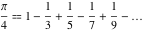 (currently named the Gregory‐Leibniz series or Leibniz formula) and evaluated π with 11 correct digits. Ghyath ad-din Jamshid Kashani (Persia, 1424) evaluated π with 16 correct digits. F. Viete (1593) represented (currently named the Gregory‐Leibniz series or Leibniz formula) and evaluated π with 11 correct digits. Ghyath ad-din Jamshid Kashani (Persia, 1424) evaluated π with 16 correct digits. F. Viete (1593) represented  as the infinite product as the infinite product 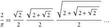 . Ludolph van Ceulen (Germany, 1610) evaluated 35 decimal places of π. J. Wallis (1655) represented . Ludolph van Ceulen (Germany, 1610) evaluated 35 decimal places of π. J. Wallis (1655) represented  as the infinite product as the infinite product 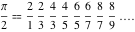 J. Machin (England, 1706) developed a quickly converging series for J. Machin (England, 1706) developed a quickly converging series for  , based on the formula , based on the formula 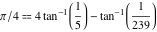 , and used it to evaluate 100 correct digits. W. Jones (1706) introduced the symbol π for notation of the Pi constant. L. Euler (1737) adopted the symbol π and made it standard. C. Goldbach (1742) also widely used the symbol π. J. H. Lambert (1761) established that π is an irrational number. J. Vega (Slovenia, 1789) improved J. Machin's 1706 formula and calculated 126 correct digits for , and used it to evaluate 100 correct digits. W. Jones (1706) introduced the symbol π for notation of the Pi constant. L. Euler (1737) adopted the symbol π and made it standard. C. Goldbach (1742) also widely used the symbol π. J. H. Lambert (1761) established that π is an irrational number. J. Vega (Slovenia, 1789) improved J. Machin's 1706 formula and calculated 126 correct digits for  . W. Rutherford (1841) calculated 152 correct digits for . W. Rutherford (1841) calculated 152 correct digits for  . After 20 years of hard work, W. Shanks (1873) presented 707 digits for . After 20 years of hard work, W. Shanks (1873) presented 707 digits for  , but only 527 digits were correct (as D. F. Ferguson found in 1947). F. Lindemann (1882) proved that π is transcendental. F. C. W. Stormer (1896) derived the formula , but only 527 digits were correct (as D. F. Ferguson found in 1947). F. Lindemann (1882) proved that π is transcendental. F. C. W. Stormer (1896) derived the formula  , which was used in 2002 for the evaluation of 1,241,100,000,000 digits of , which was used in 2002 for the evaluation of 1,241,100,000,000 digits of  . D. F. Ferguson (1947) recalculated π to 808 decimal places, using a mechanical desk calculator. K. Mahler (1953) proved that . D. F. Ferguson (1947) recalculated π to 808 decimal places, using a mechanical desk calculator. K. Mahler (1953) proved that  is not a Liouville number. is not a Liouville number.
Modern computer calculation of π was started by D. Shanks (1961), who reported 100000 digits of  . This record was improved many times; Yasumasa Kanada (Japan, December 2002) using a 64-node Hitachi supercomputer evaluated 1,241,100,000,000 digits of . This record was improved many times; Yasumasa Kanada (Japan, December 2002) using a 64-node Hitachi supercomputer evaluated 1,241,100,000,000 digits of  . For this purpose he used the earlier mentioned formula of F. C. W. Stormer (1896) and the formula . For this purpose he used the earlier mentioned formula of F. C. W. Stormer (1896) and the formula  . Future improved results are inevitable. . Future improved results are inevitable.
Babylonians divided the circle into 360 degrees (360°), probably because 360 approximates the number of days in a year. Ptolemy (Egypt, c. 90–168 AD) in Mathematical Syntaxis used the symbol sing  in astronomical calculations. Mathematically, one degree in astronomical calculations. Mathematically, one degree  has the numerical value has the numerical value 
Therefore, all historical and other information about  can be derived from information about can be derived from information about  . .
J. Napier in his work on logarithms (1618) mentioned the existence of a special convenient constant for the calculation of logarithms (but he did not evaluate this constant). It is possible that the table of logarithms was written by W. Oughtred, who is credited in 1622 with inventing the slide rule, which is a tool used for multiplication, division, evaluation of roots, logarithms, and other functions. In 1669 I. Newton published the series  , which actually converges to that special constant. At that time J. Bernoulli tried to find the limit of , which actually converges to that special constant. At that time J. Bernoulli tried to find the limit of  , when , when  . G. W. Leibniz (1690–1691) was the first, in correspondence to C. Huygens, to recognize this limit as a special constant, but he used the notation . G. W. Leibniz (1690–1691) was the first, in correspondence to C. Huygens, to recognize this limit as a special constant, but he used the notation  to represent it. to represent it.
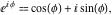
L. Euler began using the letter  for that constant in 1727–1728, and introduced this notation in a letter to C. Goldbach (1731). However, the first use of for that constant in 1727–1728, and introduced this notation in a letter to C. Goldbach (1731). However, the first use of  in a published work appeared in Euler's Mechanica (1736). In 1737 L. Euler proved that ⅇ and in a published work appeared in Euler's Mechanica (1736). In 1737 L. Euler proved that ⅇ and  are irrational numbers and represented are irrational numbers and represented  through continued fractions. In 1748 L. Euler represented through continued fractions. In 1748 L. Euler represented  as an infinite sum and found its first 23 digits: as an infinite sum and found its first 23 digits:
D. Bernoulli (1760) used  as the base of the natural logarithms. J. Lambert (1768) proved that as the base of the natural logarithms. J. Lambert (1768) proved that  is an irrational number, if is an irrational number, if  is a nonzero rational number.
In the 19th century A. Cauchy (1823) determined that is a nonzero rational number.
In the 19th century A. Cauchy (1823) determined that  ; J. Liouville (1844) proved that ; J. Liouville (1844) proved that  does not satisfy any quadratic equation with integral coefficients; C. Hermite (1873) proved that ⅇ is a transcendental number; and E. Catalan (1873) represented ⅇ through infinite products. does not satisfy any quadratic equation with integral coefficients; C. Hermite (1873) proved that ⅇ is a transcendental number; and E. Catalan (1873) represented ⅇ through infinite products.
The only constant appearing more frequently than ⅇ in mathematics is π. Physical applications of  are very often connected with time-dependent processes. For example, if are very often connected with time-dependent processes. For example, if  is a decreasing value of a quantity at time is a decreasing value of a quantity at time  , which decreases at a rate proportional to its value with coefficient , which decreases at a rate proportional to its value with coefficient  , this quantity is subject to exponential decay described by the following differential equation and its solution: , this quantity is subject to exponential decay described by the following differential equation and its solution:
where  is the initial quantity at time is the initial quantity at time  . Examples of such processes can be found in the following: a radionuclide that undergoes radioactive decay, chemical reactions (like enzyme-catalyzed reactions), electric charge, vibrations, pharmacology and toxicology, and the intensity of electromagnetic radiation. . Examples of such processes can be found in the following: a radionuclide that undergoes radioactive decay, chemical reactions (like enzyme-catalyzed reactions), electric charge, vibrations, pharmacology and toxicology, and the intensity of electromagnetic radiation.
In 1735 the Swiss mathematician L. Euler introduced a special constant that represents the limiting difference between the harmonic series and the natural logarithm:
Euler denoted it using the symbol  , and initially calculated its value to 6 decimal places, which he extended to 16 digits in 1781. L. Mascheroni (1790) first used the symbol , and initially calculated its value to 6 decimal places, which he extended to 16 digits in 1781. L. Mascheroni (1790) first used the symbol  for the notation of this constant and calculated its value to 19 correct digits. Later J. Soldner (1809) calculated for the notation of this constant and calculated its value to 19 correct digits. Later J. Soldner (1809) calculated  to 40 correct digits, which C. Gauss and F. Nicolai (1812) verified. E. Catalan (1875) found the integral representation for this constant to 40 correct digits, which C. Gauss and F. Nicolai (1812) verified. E. Catalan (1875) found the integral representation for this constant  . .
This constant was named the Euler gamma or Euler‐Mascheroni constant in the honor of its founders.
Applications include discrete mathematics and number theory.
The Catalan constant  was named in honor of Eu. Ch. Catalan (1814–1894), who introduced a faster convergent equivalent series and expressions in terms of integrals. Based on methods resulting from collaborations with M. Leclert, E. Catalan (1865) computed was named in honor of Eu. Ch. Catalan (1814–1894), who introduced a faster convergent equivalent series and expressions in terms of integrals. Based on methods resulting from collaborations with M. Leclert, E. Catalan (1865) computed  up to 9 decimals. M. Bresse (1867) computed 24 decimals of up to 9 decimals. M. Bresse (1867) computed 24 decimals of  using a technique from E. Kummer's work. J. Glaisher (1877) evaluated 20 digits of the Catalan constant, which he extended to 32 digits in 1913. using a technique from E. Kummer's work. J. Glaisher (1877) evaluated 20 digits of the Catalan constant, which he extended to 32 digits in 1913.
The Catalan constant is applied in number theory, combinatorics, and different areas of mathematical analysis.
The works of H. Kinkelin (1860) and J. Glaisher (1877–1878) introduced one special constant:
which was later called the Glaisher or Glaisher‐Kinkelin constant in honor of its founders. This constant is used in number theory, Bose‐Einstein and Fermi‐Dirac statistics, analytic approximation and evaluation of integrals and products, regularization techniques in quantum field theory, and the Scharnhorst effect of quantum electrodynamics.
The 1934 work of A. Khinchin considered the limit of the geometric mean of continued fraction terms  and found that its value is a constant independent for almost all continued fractions: and found that its value is a constant independent for almost all continued fractions:
The constant—named the Khinchin constant in the honor of its founder—established that rational numbers, solutions of quadratic equations with rational coefficients, the golden ratio  , and the Euler number , and the Euler number  upon being expanded into continued fractions do not have the previous property. Other site numerical verifications showed that continued fraction expansions of upon being expanded into continued fractions do not have the previous property. Other site numerical verifications showed that continued fraction expansions of  , the Euler-Mascheroni constant , the Euler-Mascheroni constant  , and Khinchin's constant , and Khinchin's constant  itself can satisfy that property. But it was still not proved accurately. itself can satisfy that property. But it was still not proved accurately.
Applications of the Khinchin constant  include number theory. include number theory.
The imaginary unit constant  allows the real number system allows the real number system  to be extended to the complex number system to be extended to the complex number system  . This system allows for solutions of polynomial equations such as . This system allows for solutions of polynomial equations such as  and more complicated polynomial equations through complex numbers. Hence and more complicated polynomial equations through complex numbers. Hence  and and  , and the previous quadratic equation has two solutions as is expected for a quadratic polynomial: , and the previous quadratic equation has two solutions as is expected for a quadratic polynomial:
The imaginary unit has a long history, which started with the question of how to understand and interpret the solution of the simple quadratic equation  . .
It was clear that  . But it was not clear how to get . But it was not clear how to get  from something squared. from something squared.
In the 16th, 17th, and 18th centuries this problem was intensively discussed together with the problem of solving the cubic, quartic, and other polynomial equations. S. Ferro (Italy, 1465–1526) first discovered a method to solve cubic equations. N. F. Tartaglia (Italy, 1500–1557) independently solved cubic equations. G. Cardano (Italy, 1545) published the solutions to the cubic and quartic equations in his book Ars Magna, with one case of this solution communicated to him by N. Tartaglia. He noted the existence of so-called imaginary numbers, but did not describe their properties. L. Ferrari (Italy, 1522–1565) solved the quartic equation, which was mentioned in the book Ars Magna by his teacher G. Cardano. R. Descartes (1637) suggested the name "imaginary" for nonreal numbers like  . J. Wallis (1685) in De Algebra tractates published the idea of the graphic representation of complex numbers. J. Bernoulli (1702) used imaginary numbers. R. Cotes (1714) derived the formula: . J. Wallis (1685) in De Algebra tractates published the idea of the graphic representation of complex numbers. J. Bernoulli (1702) used imaginary numbers. R. Cotes (1714) derived the formula:
|
which in 1748 was found by L. Euler and hence named for him.
A. Moivre (1730) derived the well-known formula  , which bears his name.
Investigations of L. Euler (1727, 1728) gave new imputus to the theory of complex numbers and functions of complex arguments (analytic functions). In a letter to C. Goldbach (1731) L. Euler introduced the notation ⅇ for the base of the natural logarithm ⅇ⩵2.71828182… and he proved that ⅇ is irrational. Later on L. Euler (1740–1748) found a series expansion for , which bears his name.
Investigations of L. Euler (1727, 1728) gave new imputus to the theory of complex numbers and functions of complex arguments (analytic functions). In a letter to C. Goldbach (1731) L. Euler introduced the notation ⅇ for the base of the natural logarithm ⅇ⩵2.71828182… and he proved that ⅇ is irrational. Later on L. Euler (1740–1748) found a series expansion for  , which lead to the famous and very basic formula connecting exponential and trigonometric functions , which lead to the famous and very basic formula connecting exponential and trigonometric functions 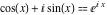 (1748). H. Kühn (1753) used imaginary numbers. L. Euler (1755) used the word "complex" (1777) and first used the letter (1748). H. Kühn (1753) used imaginary numbers. L. Euler (1755) used the word "complex" (1777) and first used the letter  to represent to represent  . C. Wessel (1799) gave a geometrical interpretation of complex numbers. . C. Wessel (1799) gave a geometrical interpretation of complex numbers.
As a result, mathematicians introduced the use of a special symbol—the imaginary unit  that is equal to that is equal to  : :
In the 19th century the conception and theory of complex numbers was basically formed. A. Buee (1804) independently came to the idea of J. Wallis about geometrical representations of complex numbers in the plane. J. Argand (1806) introduced the name modulus for  , and published the idea of geometrical interpretation of complex numbers known as the Argand diagram. C. Mourey (1828) laid the foundations for the theory of directional numbers in a little treatise. , and published the idea of geometrical interpretation of complex numbers known as the Argand diagram. C. Mourey (1828) laid the foundations for the theory of directional numbers in a little treatise.
The imaginary unit  was interpreted in a geometrical sense as the point with coordinates was interpreted in a geometrical sense as the point with coordinates  in the Cartesian (Euclidean) in the Cartesian (Euclidean)  , , plane with the vertical plane with the vertical  axis upward and the origin axis upward and the origin  . This geometric interpretation establishes the following representations of the complex number . This geometric interpretation establishes the following representations of the complex number  through two real numbers through two real numbers  and and  as: as:
where  is the distance between points is the distance between points  and and  and and  is the angle between the line connecting points is the angle between the line connecting points  and and  and the positive and the positive  axis direction (the so-called polar representation).
The last formula lead to the following basic relations: axis direction (the so-called polar representation).
The last formula lead to the following basic relations:
which describe the main characteristics of the complex number  —the so-called modulus (absolute value) —the so-called modulus (absolute value)  , the real part , the real part  , the imaginary part , the imaginary part  , and the argument , and the argument  . .
The Euler formula 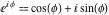 allows the representation of the complex number allows the representation of the complex number  , using polar coordinates , using polar coordinates  in the more compact form: in the more compact form:
It also allows the expression of the logarithm of a complex number through the formula:
Taking into account that the cosine and sine have period  , it follows that , it follows that  has period has period  : :
Generically, the logarithm function  is the multivalued function: is the multivalued function:
For specifying just one value for the logarithm  and one value of the argument ϕ for a given complex number and one value of the argument ϕ for a given complex number  , the restriction , the restriction  is generally used for the argument ϕ. is generally used for the argument ϕ.
C. F. Gauss (1831) introduced the name "imaginary unit" for  , suggested the term complex number for , suggested the term complex number for  , and called , and called  the norm, but mentioned that the theory of complex numbers is quite unknown, and in 1832 published his chief memoir on the subject. A. Cauchy (1789–1857) proved several important basic theorems in complex analysis. N. Abel (1802–1829) was the first to widely use complex numbers with well-known success. K. Weierstrass (1841) introduced the notation the norm, but mentioned that the theory of complex numbers is quite unknown, and in 1832 published his chief memoir on the subject. A. Cauchy (1789–1857) proved several important basic theorems in complex analysis. N. Abel (1802–1829) was the first to widely use complex numbers with well-known success. K. Weierstrass (1841) introduced the notation  for the modulus of complex numbers, which he called the absolute value. E. Kummer (1844), L. Kronecker (1845), Scheffler (1845, 1851, 1880), A. Bellavitis (1835, 1852), Peacock (1845), A. Morgan (1849), A. Mobius (1790–1868), J. Dirichlet (1805–1859), and others made large contributions in developing complex number theory. for the modulus of complex numbers, which he called the absolute value. E. Kummer (1844), L. Kronecker (1845), Scheffler (1845, 1851, 1880), A. Bellavitis (1835, 1852), Peacock (1845), A. Morgan (1849), A. Mobius (1790–1868), J. Dirichlet (1805–1859), and others made large contributions in developing complex number theory.
|