Introduction to the Cosine Function

Defining the cosine function

The cosine function is one of the oldest mathematical functions. It was first used in ancient Egypt in the book of Ahmes (c. 2000 B.C.). Much later F. Viète (1590) evaluated some values of , E. Gunter (1636) introduced the notation "Cosi" and the word "cosinus" (replacing "complementi sinus"), and I. Newton (1658, 1665) found the series expansion for .

The classical definition of the cosine function for real arguments is: "the cosine of an angle in a right‐angle triangle is the ratio of the length of the adjacent leg to the length of the hypotenuse." This description of is valid for when the triangle is nondegenerate. This approach to the cosine can be expanded to arbitrary real values of if consideration is given to the arbitrary point in the ,‐Cartesian plane and is defined as the ratio , assuming that α is the value of the angle between the positive direction of the ‐axis and the direction from the origin to the point .

The following formula can also be used as a definition of the cosine function:

This series converges for all finite numbers .

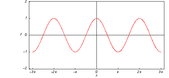
A quick look at the cosine function

Here is a graphic of the cosine function for real values of its argument .

Representation through more general functions

The function is a particular case of more complicated mathematical functions. For example, it is a special case of the generalized hypergeometric function with the parameter at :

It is also a particular case of the Bessel function with the parameter , multiplied by :

Other Bessel functions can also be expressed through cosine functions for similar values of the parameter:

Struve functions can also degenerate into the cosine function for similar values of the parameter:

But the function is also a degenerate case of the doubly periodic Jacobi elliptic functions when their second parameter is equal to or :

Finally, the function is the particular case of another class of functions—the Mathieu functions:

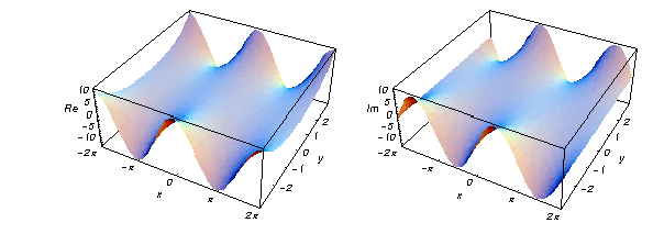
Definition of the cosine function for a complex argument

In the complex ‐plane, the function is defined using the exponential function in the points and through the formula:

The key role in this definition of belongs to the famous Euler formula that connects the exponential, the sine, and the cosine functions:

Changing to , the Euler formula can be converted into the following modification:

Adding the preceding formulas gives the following result:

Here are two graphics showing the real and imaginary parts of the cosine function over the complex plane.

The best-known properties and formulas for the cosine function

Values in points

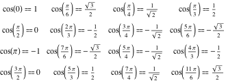
Students usually learn the following basic table of cosine function values for special points of the circle:

General characteristics

For real values of argument , the values of are real.

In the points , the values of are algebraic. In several cases they can even be rational numbers, 0, or 1. Here are some examples:

The values of can be expressed using only square roots if and is a product of a power of 2 and distinct Fermat primes {3, 5, 17, 257, …}.

The function is an entire analytical function of that is defined over the whole complex ‐plane and does not have branch cuts and branch points. It has an essential singular point at . It is a periodic function with the real period :

The function is an even function with mirror symmetry:

Differentiation

The derivatives of have simple representations using either the function or the function:

Ordinary differential equation

The function satisfies the simplest possible linear differential equation with constant coefficients:

The complete solution of this equation can be represented as a linear combination of and with arbitrary constant coefficients and :

The function also satisfies first-order nonlinear differential equations:

Series representation

The function has a simple series expansion at the origin that converges in the whole complex ‐plane:

For real this series can be interpreted as the real part of the series expansion for the exponential function :

Product representation

The following famous infinite product representation for clearly illustrates that at :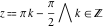

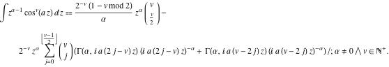
Indefinite integration

Indefinite integrals of expressions involving the cosine function can sometimes be expressed using elementary functions. However, special functions are frequently needed to express the results even when the integrands have a simple form (if they can be evaluated in closed form). Here are some examples:

The last integral cannot be evaluated in closed form using the known classical special functions for arbitrary values of parameters and .

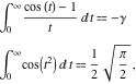
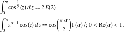
Definite integration

Definite integrals that contain the cosine function are sometimes simple. For example, the famous Dirichlet type and Fresnel integrals have the following values:

where is the Euler‐Mascheroni constant .

Some special functions can be used to evaluate more complicated definite integrals. For example, elliptic integrals and gamma functions are needed to express the following integrals:

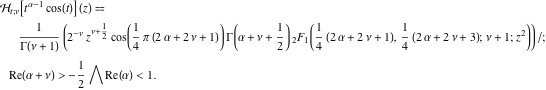
Integral transforms

Integral transforms of expressions involving the cosine function may not be classically convergent but can be interpreted in a generalized functions (distributions) sense. For example, the exponential Fourier transform of the cosine function does not exist in the classical sense but can be expressed using the Dirac delta function.

Among other integral transforms of the cosine function, the best known are the Fourier cosine and sine transforms, and the Laplace, Mellin, Hilbert, and Hankel transforms:

Finite summation

The following finite sums from the cosine can be expressed using the trigonometric functions:

Infinite summation

The following infinite sums can be expressed using elementary functions:

Finite products

The following finite products from the cosine can be expressed using trigonometric functions:

Infinite products

The following infinite product that contains the cosine function can be expressed using the sine function:

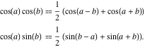
Addition formulas

The cosine of a sum can be represented by the rule: "the cosine of a sum is equal to the product of the cosines minus the product of the sines." A similar rule is valid for the cosine of the difference:

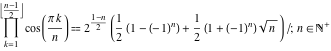
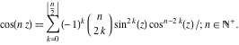
Multiple arguments

In the case of multiple arguments , , , …, the function can be represented as the finite sum of terms that include powers of the sine and the cosine:

The function can also be represented as the finite sum including only the cosine of :

Half-angle formulas

The cosine of the half‐angle can be represented by the following simple formula that is valid in some vertical strips:

To make this formula correct for all complex , a complicated prefactor is needed:

where contains the unit step, real part, imaginary part, and the floor functions.

Sums of two direct functions

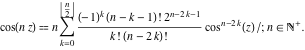
The sum of two cosine functions can be described by the rule: "the sum of the cosines is equal to two times the cosine of the half‐difference multiplied by the cosine of the half‐sum." A similar rule is valid for the difference of two cosines:

Products involving the direct function

The product of two cosine functions and the product of the cosine and sine have the following representations:

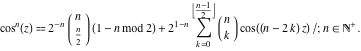
Powers of the direct function

The integer powers of the cosine functions can be expanded as finite sums of cosine functions with multiple arguments. These sums include binomial coefficients:

Inequalities

The best-known inequalities for cosine functions are the following:

Relations with its inverse function

There are simple relations between the function and its inverse function :

The second formula is valid at least in the vertical strip . Outside of this strip, a much more complicated relation (that contains the unit step, real part, and the floor functions) holds:

Representations through other trigonometric functions

Cosine and sine functions are connected by a very simple formula including the linear function in the argument:

Another famous formula, connecting and , is shown in the well‐known Pythagorean theorem:

The last restriction on can be removed, but the formula will get a complicated coefficient with , that contains the unit step, real part, imaginary part, and the floor function:

The cosine function can also be represented using other trigonometric functions by the following formulas:

Representations through hyperbolic functions

The cosine function has representations using the hyperbolic functions:

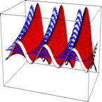
Applications

The cosine function is used throughout mathematics, the exact sciences, and engineering.